Note
Go to the end to download the full example code.
Postprocess a static mechanical simulation#
This example shows how to postprocess a static mechanical simulation to extract results like displacement and stress. It shows how to select subparts of the results by scoping on specific nodes or elements.
Note
This example requires DPF 3.0 (2022 R1) or above. For more information, see PyDPF library compatibilities.
Perform required imports#
Perform required imports. This example uses a supplied file that you can
get by importing the DPF examples package.
from ansys.dpf import post
from ansys.dpf.post import examples
Get Simulation object#
Get the Simulation object that allows access to the result. The Simulation
object must be instantiated with the path for the result file. For example,
"C:/Users/user/my_result.rst" on Windows or "/home/user/my_result.rst"
on Linux.
example_path = examples.find_static_rst()
# to automatically detect the simulation type, use:
simulation = post.load_simulation(example_path)

# to enable auto-completion, use the equivalent:
simulation = post.StaticMechanicalSimulation(example_path)

# print the simulation to get an overview of what's available
print(simulation)

displacement = simulation.displacement()
print(displacement)
Static Mechanical Simulation.


Data Sources
------------------------------
/opt/hostedtoolcache/Python/3.10.20/x64/lib/python3.10/site-packages/ansys/dpf/core/examples/result_files/static.rst

DPF Model
------------------------------
Static analysis
Unit system: MKS: m, kg, N, s, V, A, degC
Physics Type: Mechanical
Available results:
     -  node_orientations: Nodal Node Euler Angles
     -  displacement: Nodal Displacement
     -  reaction_force: Nodal Reaction Force
     -  stress: ElementalNodal Stress
     -  elemental_volume: Elemental Volume
     -  stiffness_matrix_energy: Elemental Energy-stiffness matrix
     -  artificial_hourglass_energy: Elemental Hourglass Energy
     -  kinetic_energy: Elemental Kinetic Energy
     -  co_energy: Elemental co-energy
     -  incremental_energy: Elemental incremental energy
     -  thermal_dissipation_energy: Elemental thermal dissipation energy
     -  elastic_strain: ElementalNodal Strain
     -  elastic_strain_eqv: ElementalNodal Strain eqv
     -  element_orientations: ElementalNodal Element Euler Angles
     -  structural_temperature: ElementalNodal Structural temperature
------------------------------
DPF  Meshed Region:
  81 nodes
  8 elements
  Unit: m
  With solid (3D) elements
------------------------------
DPF  Time/Freq Support:
  Number of sets: 1
Cumulative     Time (s)       LoadStep       Substep
1              1.000000       1              1


             results       U (m)
             set_ids           1
 node_ids components
        1          X -3.3190e-22
                   Y -6.9357e-09
                   Z -3.2862e-22
       26          X  2.2303e-09
                   Y -7.1421e-09
                   Z -2.9208e-22
      ...        ...         ...
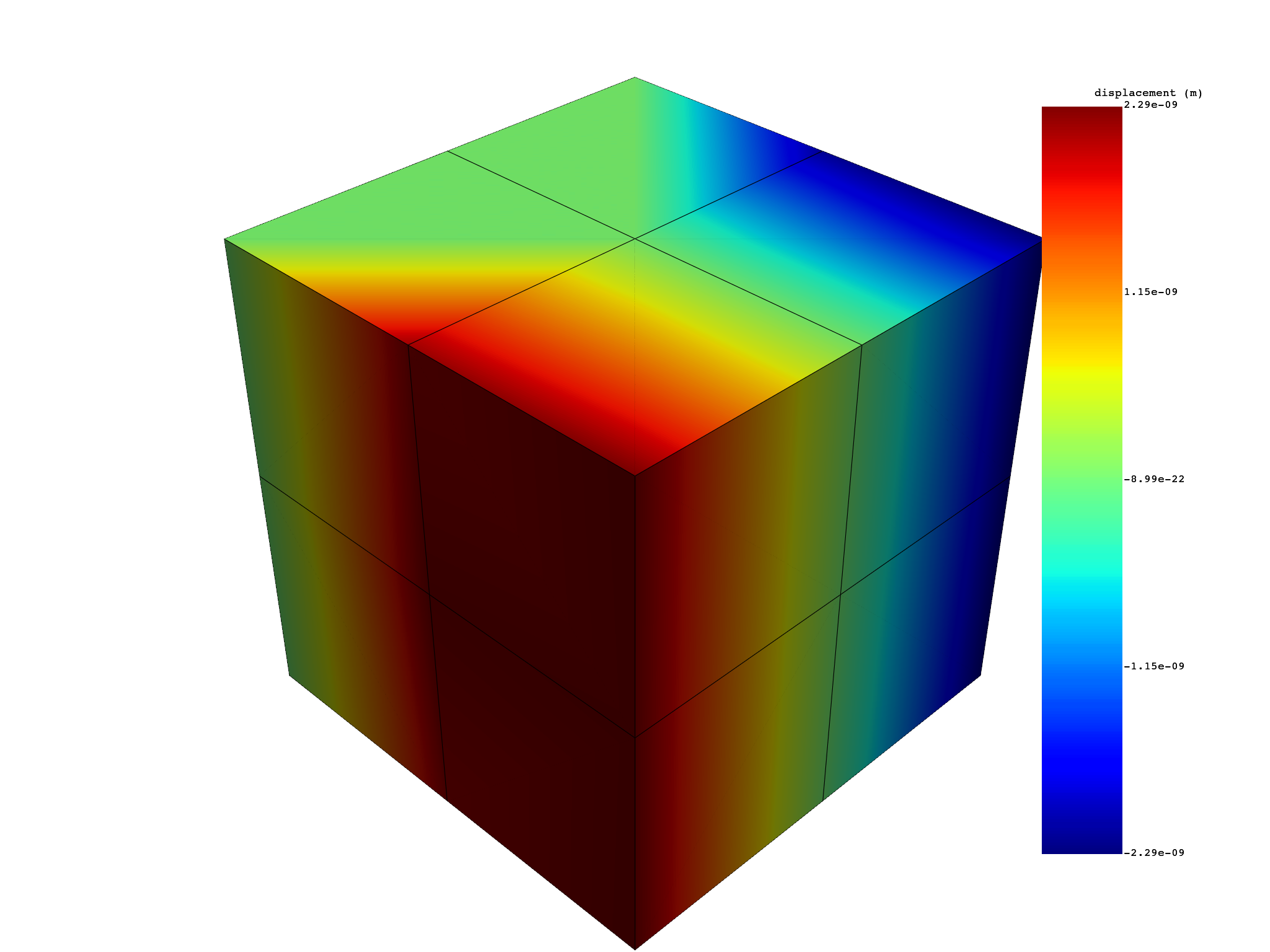
Select subparts of displacement#
# To get X displacements
x_displacement = displacement.select(components="X")
print(x_displacement)
# equivalent to
x_displacement = simulation.displacement(components=["X"])
print(x_displacement)
# plot
x_displacement.plot()
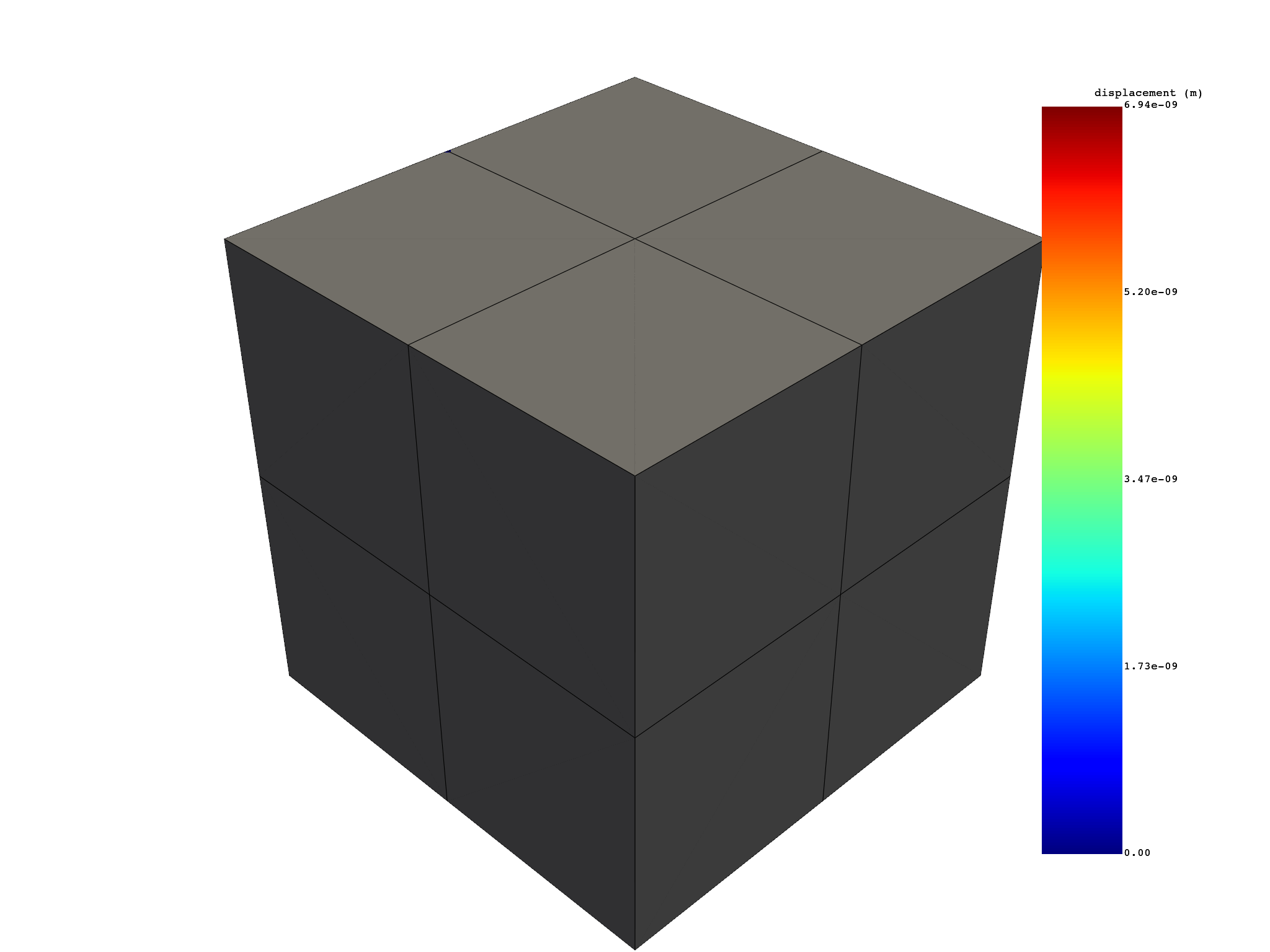
# extract displacement on specific nodes
nodes_displacement = displacement.select(node_ids=[1, 10, 100])
nodes_displacement.plot()
# equivalent to:
nodes_displacement = simulation.displacement(node_ids=[1, 10, 100])
print(nodes_displacement)
            results       U (m)
            set_ids           1
node_ids components
       1          X -3.3190e-22
      26             2.2303e-09
      14             0.0000e+00
      12             0.0000e+00
       2            -3.0117e-22
      27             2.0908e-09
     ...        ...         ...


 results     U_X (m)
 set_ids           1
node_ids
       1 -3.3190e-22
      26  2.2303e-09
      14  0.0000e+00
      12  0.0000e+00
       2 -3.0117e-22
      27  2.0908e-09
     ...         ...


            results       U (m)
            set_ids           1
node_ids components
       1          X -3.3190e-22
                  Y -6.9357e-09
                  Z -3.2862e-22
      10          X  0.0000e+00
                  Y  0.0000e+00
                  Z  0.0000e+00
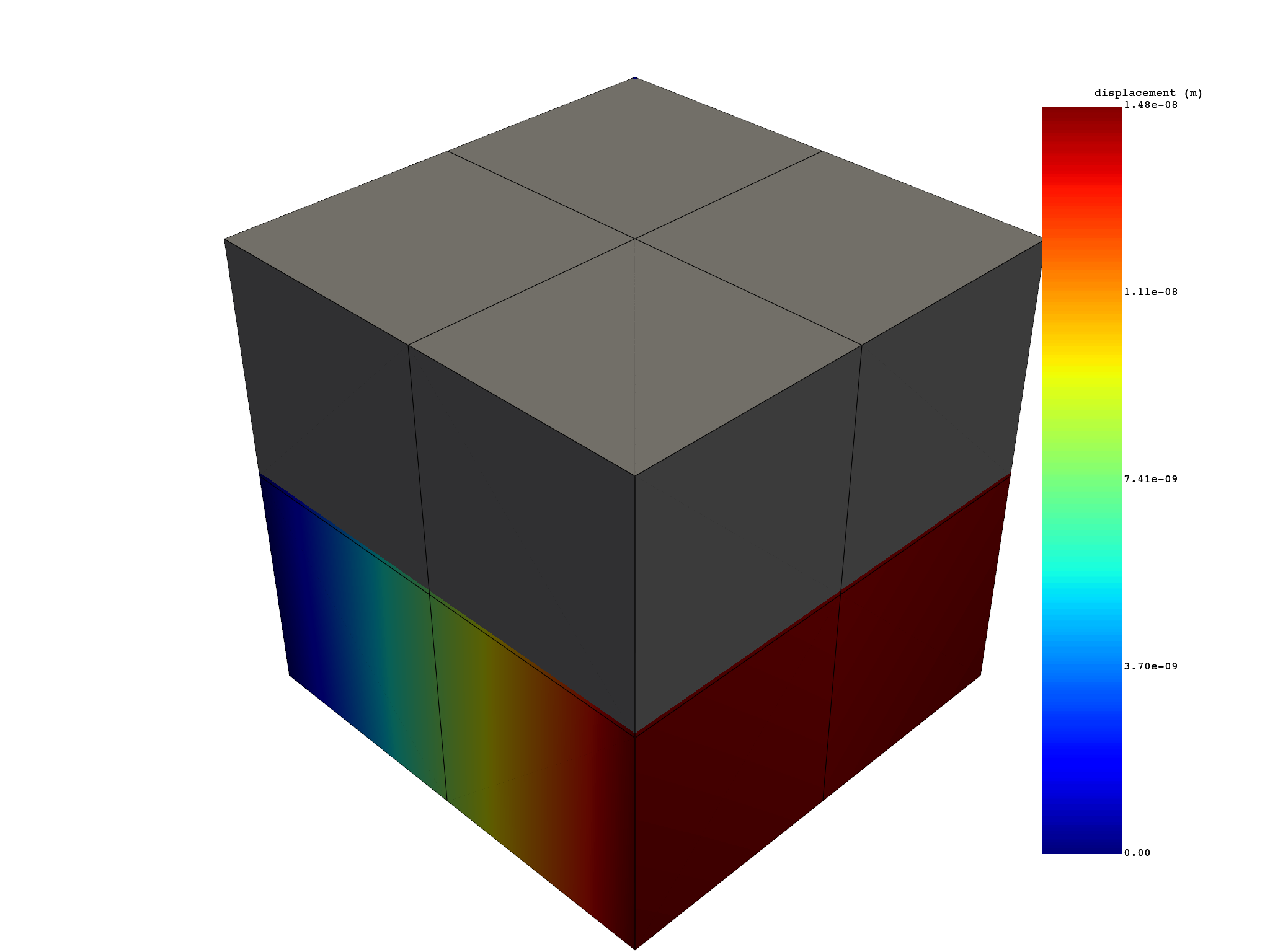
Compute total displacement (norm)#
Compute the norm of the displacement on a selection of nodes.
nodes_displacement = simulation.displacement(
    node_ids=simulation.mesh.node_ids[10:], norm=True
)
print(nodes_displacement)
nodes_displacement.plot()
  results    U_N (m)
  set_ids          1
 node_ids
       11 0.0000e+00
       12 0.0000e+00
       13 0.0000e+00
       14 0.0000e+00
       15 0.0000e+00
       16 0.0000e+00
      ...        ...


(None, <pyvista.plotting.plotter.Plotter object at 0x7f2d086655a0>)
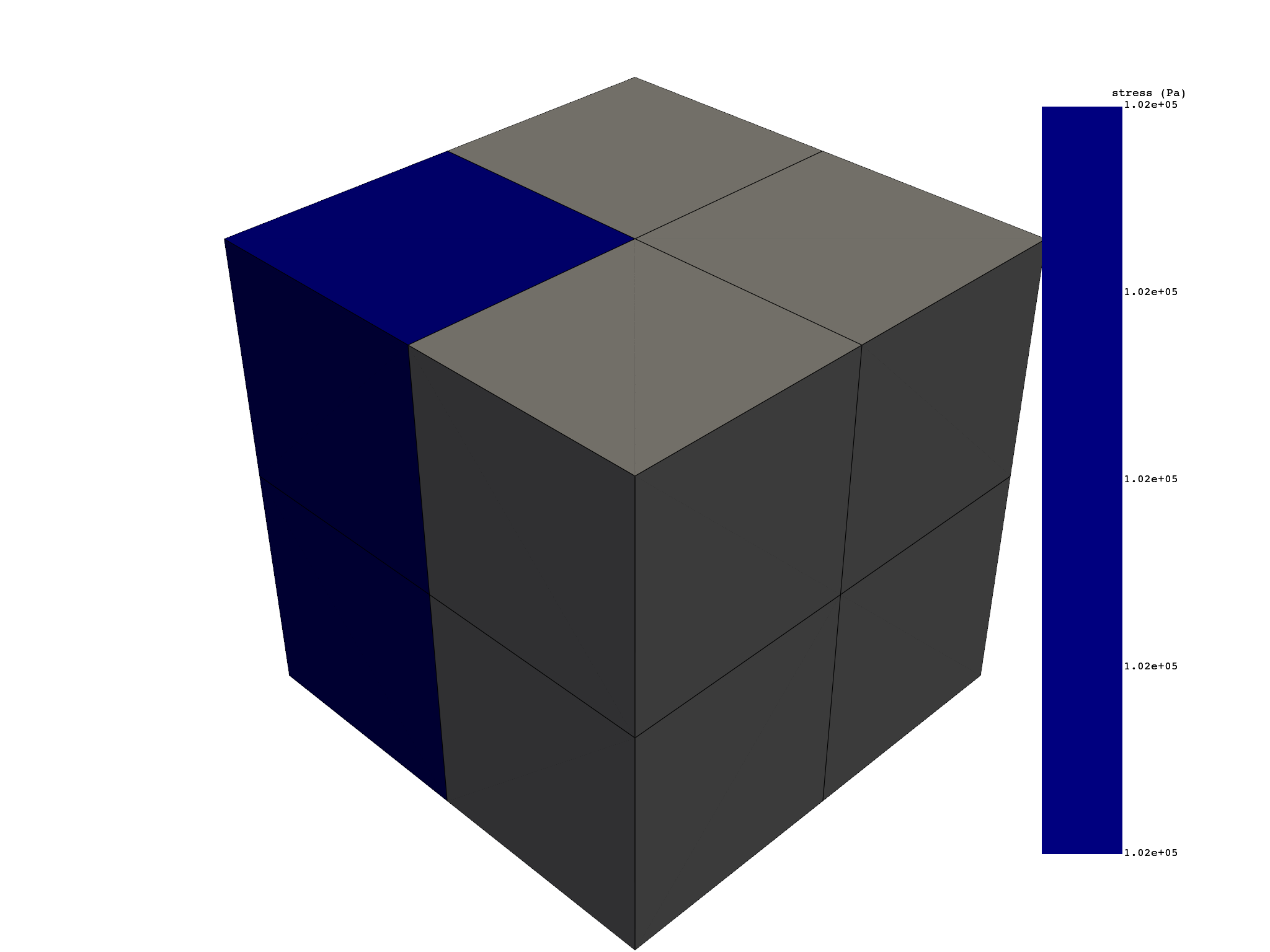
Extract tensor stresses#
Extract raw elemental nodal stresses from the result file. Then, apply averaging and compute equivalent stresses.
elem_nodal_stress = simulation.stress()
print(elem_nodal_stress)
# Compute nodal stresses from the result file
nodal_stress = simulation.stress_nodal()
print(nodal_stress)
# Compute elemental stresses from the result file
elemental_stress = simulation.stress_elemental()
print(elemental_stress)
# Extract elemental stresses on specific elements
elemental_stress = elemental_stress.select(element_ids=[5, 6, 7])
elemental_stress.plot()
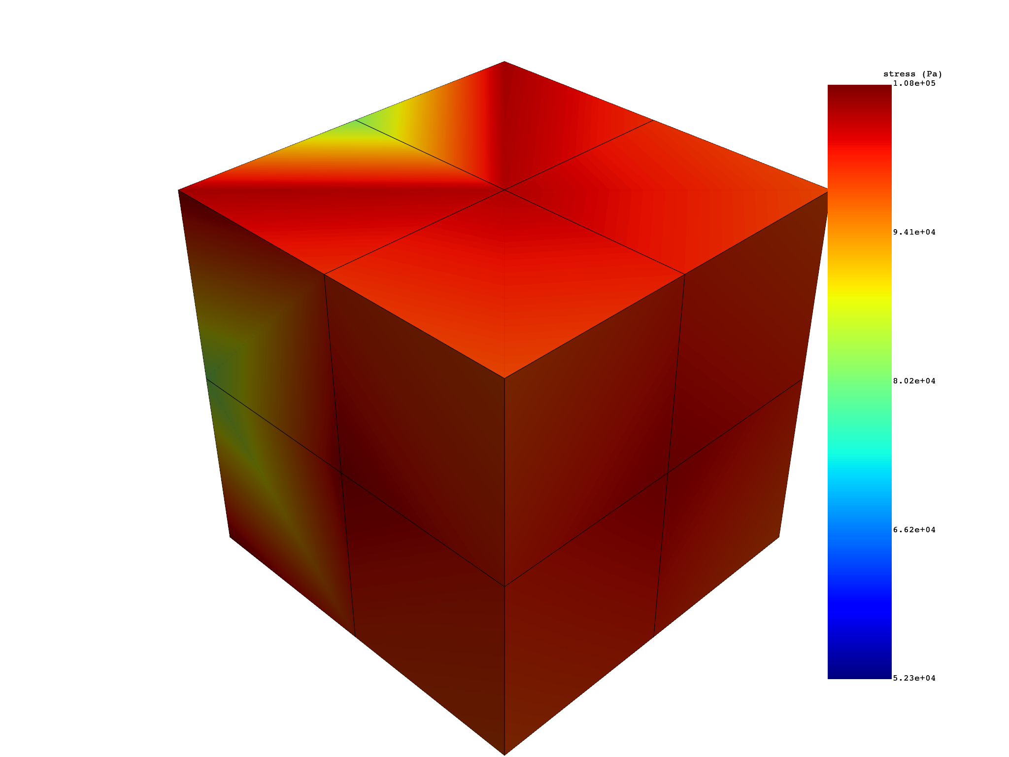
# Compute nodal eqv stresses from the result file
eqv_stress = simulation.stress_eqv_von_mises_nodal()
print(eqv_stress)
eqv_stress.plot()
                results      S (Pa)                                                             ...
                set_ids           1                                                             ...
                   node           0           1           2           3           4           5 ...
 element_ids components                                                                         ...
           5         XX -3.7836e+03  1.1793e+04 -3.2947e+04 -2.2019e+04  7.3721e+03  1.8301e+04 ...
                     YY -1.2110e+05 -9.9179e+04 -1.0033e+05 -7.4344e+04 -9.9179e+04 -8.0542e+04 ...
                     ZZ -3.7836e+03  7.3721e+03 -3.2461e+04 -2.2019e+04  1.1793e+04  1.8301e+04 ...
                     XY  5.3318e+02 -9.7301e+03  2.6037e+04 -1.2541e+03  5.5354e+02 -1.1500e+04 ...
                     YZ -5.3318e+02 -5.5354e+02  1.1343e+03  1.2541e+03  9.7301e+03  1.1500e+04 ...
                     XZ -1.4540e+02  5.9879e+02 -2.4309e+02 -2.1037e-10  5.9879e+02  2.5527e+02 ...
         ...        ...         ...         ...         ...         ...         ...         ... ...


             results      S (Pa)
             set_ids           1
 node_ids components
        1         XX -4.8113e+03
                  YY -1.1280e+05
                  ZZ -4.8113e+03
                  XY  0.0000e+00
                  YZ  0.0000e+00
                  XZ  0.0000e+00
      ...        ...         ...


                results      S (Pa)
                set_ids           1
 element_ids components
           5         XX -1.2071e+04
                     YY -1.0000e+05
                     ZZ -1.2071e+04
                     XY  3.8006e+03
                     YZ -3.8006e+03
                     XZ  4.1885e+01
         ...        ...         ...


  results  S_VM (Pa)
  set_ids          1
 node_ids
        1 1.0799e+05
       26 1.0460e+05
       14 8.1283e+04
       12 5.2324e+04
        2 1.0460e+05
       27 1.0006e+05
      ...        ...


(None, <pyvista.plotting.plotter.Plotter object at 0x7f2cd39581c0>)
Total running time of the script: (0 minutes 7.620 seconds)